The Deviation of China Map as a Regression Problem

Wu Yongzheng

1 Introduction

2 Notation

We need to find out two functions, fx(x,y) and fy(x,y), to describe the deviation. x and y are the true longitude and latitude respectively. fx(x,y) and fy(x,y) are the deviation delta at point (x,y). In other words, if (x,y) is the true coordinate, then (x + fx(x,y),y + fy(x,y)) is the deviated coordinate. Since |fx(x + d,y) -fx(x,y)| is much smaller than d (and same for y) we can also use the two functions to calculate the true coordinate from a deviated coordinate. Let (x,y) be the deviated coordinate, (x - fx(x,y),y - fy(x,y)) is the true coordinate.

In the following analysis, we will use octave. All the data used in the analysis has already been posted in my previous article1 .

3 The four 1D cases

We first solve the functions in one dimension by setting one parameter to be constant. I.e. instead of solving fx(x,y) directly, we first solve fx(x,c) and fx(c,y), where c is a constant. For example, we will look at fx(x,39.36) and fx(110.16,y). Similarly, we will solve fy(x,c) and fy(c,y) before fy(x,y). In total, there are four 1D cases.

3.1 fx(const,y)

fx(const,y) looks like to be the simplest, so we solve it first.

> data=load("-ascii", "iny-f-110.txt");
> y=data(:,2);
> dx=data(:,3);
> plot(y,dx) Figure 1(left)


PIC PIC


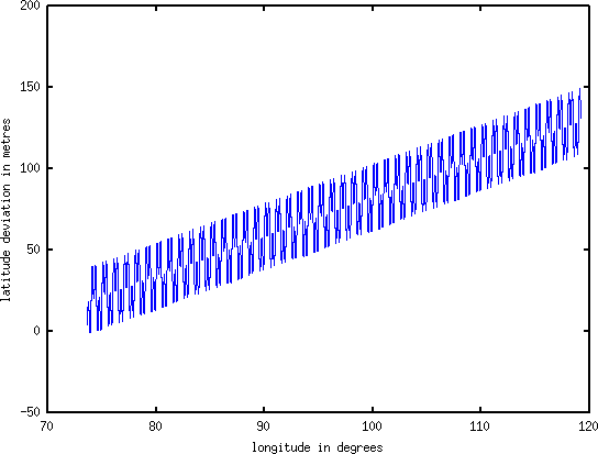
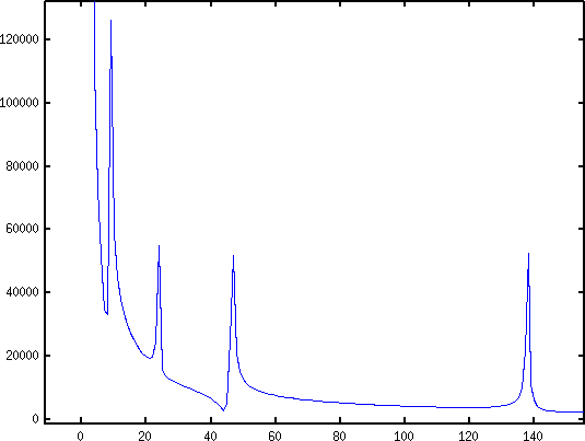
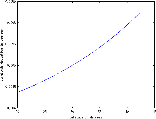
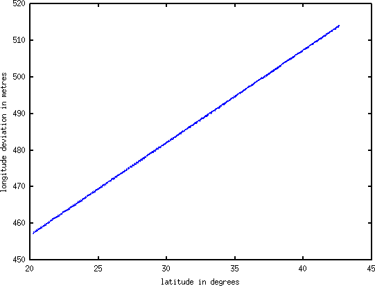
Figure 1: fx(110.16,y). Left: longitude deviation (y-axis) is in degrees; right: in metres.


Figure 1(left) shows the plot, fx(110.16,y). The curve looks like a second order curve, but if we go that direction, it’s going to be very tough. It is a lot simpler if we measure the deviation in meters rather than degrees. Note that earth’s radius is 6378137 meters in Google Map. I didn’t know this until the experiment was all finished. However, this shouldn’t cause any error even if I set the radius to 1 meter, because in the end, meters is converted back to degrees and the error cancels.

> plot(y,dx.*cos(y./180.*pi).*6371000.*pi./180) Figure 1(right)

Figure 1(right) shows the plot where the deviation is measured in meters. It’s a linear function, thus we can do a simple linear regression.

> dx=dx.*cos(y./180.*pi).*6371000.*pi./180;  
> mx=[ones(size(y)),y]; std(mx*(pinv(mx)*dx)-dx)  
ans =  0.14664  
> pinv(mx)*dx  
ans =  
   406.3954  
     2.5241

The standard error, 0.14664 meter, is acceptable, because the input data’s resolution is about 0.6 meter2 on average. The final function is

f (110.16,y) = 406.3954 + 2.5241y
 x
(1)

After trying out other constant longitudes, we find out that the two coefficients are different for different longitude. We have

fx(x,y) = g1(x) + g2(x)× y
(2)

where g1(x) and g2(x) are not yet known.

In the following analysis, we will measure x and y in degrees, while measure fx(x,y) and fy(x,y) in meters. It makes our life a lot easier.

3.2 fy(x,const)

fy(x,const) seems to be the second easiest one. It’s quite obvious that there are sinusoidal and linear components in the function. To find out the frequency of the sinusoidal components, we do a Fourier transform.

> data=load("-ascii", "inx-f-39.txt");  
> x=data(:,1);  
> size(x)  
ans =  
   9116      1  
> x(1)  
ans =  73.655  
> x(9116)  
ans =  119.23  
> dy=data(:,4).*(6371000*pi/180);

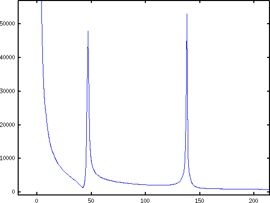
> plot(x,dy) Figure 2(left)
> plot(abs(fft(dy))) Figure 2(right)


PIC PIC


Figure 2: fy(x,39.36). Left: the data points; right: FFT of the data


Figure 2(left) shows the data and Figure 2(right) shows the data in frequency domain. The two peaks in the frequency domains are at 47 and 138, thus the frequencies are 46/45.575=1.0093 and 137/45.575=3.0060, where 45.575=119.23-73.655 is the range of x. Since the range of x is not multiple of the periods, we don’t get exact results, but after cutting the range, the exact results are 1 and 3. We then try to model it using b + kx + a1sin(2πx) + a2cos(2πx) + a3cos(6πx) + a4cos(6πx).

> mx=[ones(size(x)),x,sin(2.*pi.*x),cos(2.*pi.*x),sin(6.*pi.*x),\  
  cos(6.*pi.*x)];  
> std(mx*(pinv(mx)*dy)-dy)  
ans =  0.38114

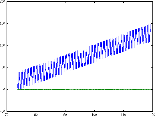
> plot(x,dy,x,dy-mx*(pinv(mx)*dy)) Figure 3


PIC


Figure 3: The data (blue) and the regression error (green).


The standard error, 0.38114, is acceptable. We can also see this in Figure 3. The regression error (difference between the data and our function) is close to zero. Let’s see the coefficients:

> pinv(mx)*dy  
ans =  
  -160.45195  
     2.42764  
    13.33287  
    -0.27150  
    13.30099  
    -0.82075

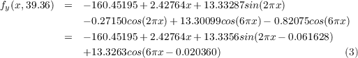
We can combine sin and cos of the same frequency.

> atan(-0.82075/13.30099)  
ans =  -0.061628  
> atan(-0.27150/13.33287)  
ans =  -0.020360  
> mx=[ones(size(x)),x,sin(2.*pi.*x-0.020360),sin(6.*pi.*x-0.061628)];  
> std(mx*(pinv(mx)*dy)-dy)  
ans =  0.38114  
> pinv(mx)*dy  
ans =  
  -160.4519  
     2.4276  
    13.3356  
    13.3263

So the function is

fy(x,39.36)  =  - 160.45195+ 2.42764x + 13.33287sin(2πx )
               - 0.27150cos(2πx) + 13.30099cos(6πx) - 0.82075cos(6πx)
            =  - 160.45195+ 2.42764x + 13.3356sin(2πx - 0.061628)
               +13.3263cos(6πx - 0.020360)                      (3)

After trying out other constant latitudes, we find out that the first two coefficients to be changing but the last 4 coefficients to be fixed. Thus, we know

fy(x,y) =   g1(y)+ g2(y)x+ 13.3356sin(2πx- 0.061628)
            +13.3263cos(6πx- 0.020360)                  (4)
where g1(y) and g2(y) are not yet known.

3.3 fx(x,const)

Similar to previous one, we use Fourier transform to find out the sinusoidal components first.

> data=load("-ascii", "inx-f-39.txt");  
> x=data(:,1);  
> dx=data(:,3).*cos(39.36./180.*pi).*6371000.*pi./180;

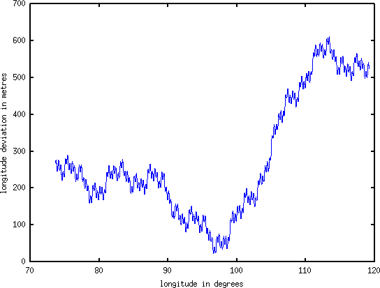
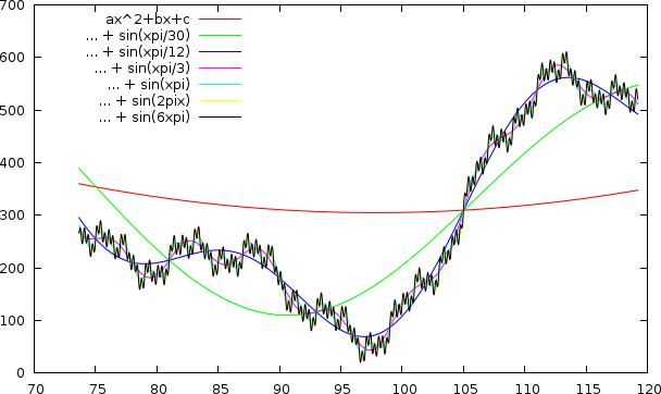
> plot(x,dx) Figure 4(left)
> plot(abs(fft(dx))) Figure 4(right)


PIC PIC


Figure 4: fx(x,39.36). Left: the data points; right: FFT of the data


Figure 4(left) shows the curve that we are going to fit. Figure 4(right) shows the frequency domain. The peaks are at 9, 24, 47 and 138, so the frequencies are 8/45.575=0.17553, 23/45.575=0.50466, 46/45.575=1.0093 and 137/45.575=3.0060. The exact frequencies are 1/6, 1/2, 1 and 3. Now, we try to fit the curve with the 4 sinusoidal components and a linear component.

> mx=[ones(size(x)),x,sin(pi.*x./3),cos(pi.*x./3),sin(pi.*x),\  
  cos((pi.*x)),sin(2.*pi.*x),cos(2.*pi.*x),sin(6.*pi.*x),\  
  cos((6.*pi.*x))]; std(mx*(pinv(mx)*dx)-dx)  
ans =  119.96  
> plot(x,dx,x,dx-mx*(pinv(mx)*dx))


PIC


Figure 5: The data (blue) and the regression error (green).


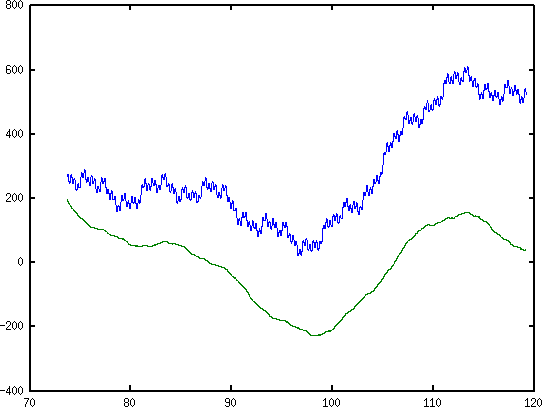
The standard error 119.96 meters is not acceptable. To see it, we plot the difference in Figure 5. It seems that there are some low frequency components. We can deal with low frequency components with a bunch of polynomials.

> mx=[ones(size(x)),(x./mean(x)),(x./mean(x)).^2,(x./mean(x)).^3,\  
  (x./mean(x)).^4,(x./mean(x)).^5,(x./mean(x)).^6,(x./mean(x)).^7,\  
  (x./mean(x)).^8,(x./mean(x)).^9,sin(pi.*x./3),cos(pi.*x./3),\  
  sin(pi.*x),cos((pi.*x)),sin(2.*pi.*x),cos(2.*pi.*x),sin(6.*pi.*x),\  
  cos((6.*pi.*x))]; std(mx*(pinv(mx)*dx)-dx)  
ans =  0.78555

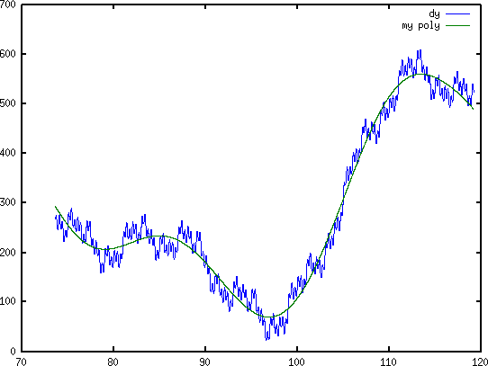
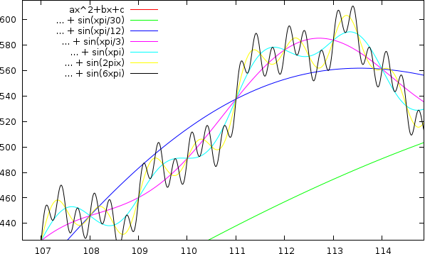
It fits well with a 9-order polynomial. Note that we divide x by mean(x) to make sure the values in the matrix have low dynamic range so as to reduce numeric error. Mathematically, they don’t make a difference. To see how our polynomial works, we can plot the polynomial and compare with the data (see Figure 6).

> coeff=pinv(mx)*dx;  
> coeff(11:18)=0  
coeff =  
   1.3529e+08  
  -1.3862e+09  
   6.2344e+09  
  -1.6167e+10  
   2.6655e+10  
  -2.8993e+10  
   2.0816e+10  
  -9.5166e+09  
   2.5150e+09  
  -2.9286e+08  
   0.0000e+00  
   0.0000e+00  
   0.0000e+00  
   0.0000e+00  
   0.0000e+00  
   0.0000e+00  
   0.0000e+00  
   0.0000e+00  
> plot(x,dx,x,mx*coeff)


PIC


Figure 6: 9-order polynomial (green) and 9-order polynomial + sinusoidal (blue)


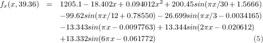
Although the 9-order polynomial fits the data well (error is 0.79 meters), the function is ugly. After lots of tries3 , I figured out that the low frequency component actually consists of a quadratic curve and two sinusoidal wave of period 60 and 24. Using this model, the regression error is 0.39 meters and the function is simple and beautiful.

> mx=[ones(size(x)),x,x.*x,sin(pi.*x./30),cos(pi.*x./30),\  
  sin(pi.*x./12),cos(pi.*x./12),sin(pi.*x./3),cos(pi.*x./3),\  
  sin(pi.*x),cos((pi.*x)),sin(2.*pi.*x),cos(2.*pi.*x),sin(6.*pi.*x),\  
  cos((6.*pi.*x))]; std(mx*(pinv(mx)*dx)-dx)  
ans =  0.38668  
> pinv(mx)*dx  
ans =  
   1.2052e+03  
  -1.8404e+01  
   9.4022e-02  
   8.3824e-01  
   2.0044e+02  
  -7.0435e+01  
  -7.0449e+01  
  -2.6699e+01  
   9.1218e-02  
  -1.3342e+01  
   1.3044e-01  
   1.3342e+01  
  -2.7504e-01  
   1.3306e+01  
  -8.2298e-01

Now let’s merge sin and cos.
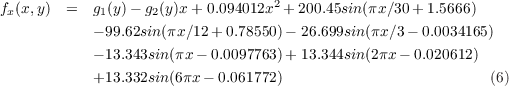
> atan(2.0044e+02/8.3824e-01)  
ans =  1.5666  
> atan(-7.0449e+01/-7.0435e+01)  
ans =  0.78550  
> atan(9.1218e-02/-2.6699e+01)  
ans =  -0.0034165  
> atan(1.3044e-01/-1.3342e+01)  
ans =  -0.0097763  
> atan(-2.7504e-01/1.3342e+01)  
ans =  -0.020612  
> atan(-8.2298e-01/1.3306e+01)  
ans =  -0.061772  
> mx=[ones(size(x)),x,x.*x,sin(pi.*x./30+1.5666),sin(pi.*x./12+0.78550),\  
  sin(pi.*x./3-0.0034165),sin(pi.*x-0.0097763),sin(2.*pi.*x-0.020612),\  
  sin(6.*pi.*x-0.061772)]; std(mx*(pinv(mx)*dx)-dx)  
ans =  0.38668  
> pinv(mx)*dx  
ans =  
   1.2051e+03  
  -1.8402e+01  
   9.4012e-02  
   2.0045e+02  
  -9.9620e+01  
  -2.6699e+01  
  -1.3343e+01  
   1.3344e+01  
   1.3332e+01

Finally, we have

f (x,39.36)  =  1205.1 - 18.402x+ 0.094012x2 + 200.45sin(πx∕30+ 1.5666)
 x
               - 99.62sin (πx ∕12 + 0.78550)- 26.699sin(πx∕3- 0.0034165)
               - 13.343sin (πx - 0.0097763)+ 13.344sin(2πx- 0.020612)
               +13.332sin (6πx - 0.061772)                        (5)
To see how the components fit the data, we can graduately add the higher frequency components. Figure 5.5 shows this this idea. Figure 5.6 is a zoomed in region in Figure 5.5. The first function (in red) is the quadratic function 1205.1 - 18.402x + 0.094012x2. The second function (in green) adds one sinusoidal component to it: 1205.1 - 18.402x + 0.094012x2 + 200.45sin(πx∕30 + 1.5666). The third function (in blue) adds one more sinusoidal component to it, etc.

PIC PIC


Figure 7: Decomposition of Components. Left: overall; right: zoomed in. The first function (red) has only the lowest frequency component. The second function (green) adds the second lowest frequency component to the first function. The third (blue) adds another component, etc.


After trying out other constant latitude, we found that only the first two coefficients are affected by latitude. The rest of the coefficients do not change. Thus, we have

fx(x,y)  =  g1(y)- g2(y)x + 0.094012x2 + 200.45sin(πx∕30+ 1.5666)
           - 99.62sin(πx∕12+ 0.78550)- 26.699sin(πx∕3 - 0.0034165)

           - 13.343sin(πx- 0.0097763)+ 13.344sin(2πx - 0.020612)
           +13.332sin(6πx- 0.061772)                          (6)
where g1(y) and g2(y) are not yet known.

3.4 fy(const,y)

The process of finding fy(const,y) is similar to fx(x,const), except that the two high frequency sinusoidal components do not appear in fy(const,y).

> data=load("-ascii", "iny-a-110.txt");  
> y=data(:,2);  
> dy=data(:,4).*(6371000*pi/180);  
> my=[ones(size(y)),y,y.*y,sin(pi.*y./30),cos(pi.*y./30),\  
  sin(pi.*y./12),cos(pi.*y./12),sin(pi.*y./3),cos(pi.*y./3),\  
  sin(pi.*y),cos((pi.*y))]; std(my*(pinv(my)*dy)-dy)  
ans =    0.16683  
> pinv(my)*dy  
ans =  
       162.1  
     -22.422  
     0.41569  
     -172.78  
      56.189  
     -104.96  
     -29.351  
      13.251  
      23.113  
     -13.357  
   -0.061311  
> atan(56.189/-172.78)  
ans =   -0.31442  
> atan(-29.351/-104.96)  
ans =    0.27267  
> atan(23.113/13.251)  
ans =     1.0502  
> atan(-0.061311/-13.357)  
ans =  0.0045901  
> my=[ones(size(y)),y,y.*y,sin(pi.*y./30-0.31442),\  
  sin(pi.*y./12+0.27267),sin(pi.*y./3+1.0502),\  
  sin(pi.*y+0.0045901)]; std(my*(pinv(my)*dy)-dy)  
ans =    0.16683  
> pinv(my)*dy  
ans =  
      162.09  
     -22.422  
     0.41568  
     -181.69  
     -108.99  
      26.643  
     -13.357

We have

                                       2
fy(110.16,y) =   162.09- 22.422y + 0.41568y
                - 181.69sin(πy∕30- 0.31442) - 108.99sin(πy∕12 +0.27267)
                +26.643sin(πy∕3+ 1.05)- 13.357sin (πy - 0.00459)    (7)
    f (x,y) =   g(x)+ g (x)y+ 0.41568y2
     y          1      2
                - 181.69sin(πy∕30- 0.31442) - 108.99sin(πy∕12 +0.27267)
                +26.643sin(πy∕3+ 1.05)- 13.357sin (πy - 0.00459)    (8)

4 The final 2D case: fx(x,y) and fy(x,y)

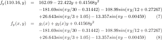
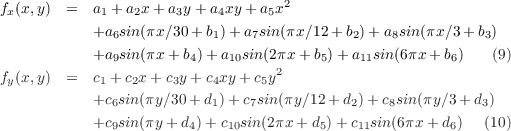
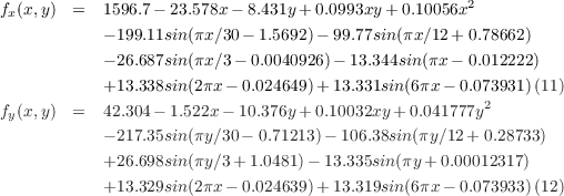
From Equation 6 and 2 we know that fx(x,y) must be in the form of Equation 9. Similarly, from Equation 4 and 8 we know fy(x,y) must be in the form of Equation 10. What’s left now is to determine the parameters.

                                   2
fx(x,y)  =  a1 + a2x + a3y + a4xy+ a5x
           +a6sin(πx∕30+ b1)+ a7sin (πx ∕12+ b2) + a8sin(πx∕3+ b3)
           +a9sin(πx +b4)+ a10sin (2πx + b5) + a11sin(6πx+ b6)   (9)
f(x,y)  =  c + c x+ c y+ c xy+ c y2
 y          1   2    3    4     5
           +c6sin(πy∕30+ d1)+ c7sin(πy∕12 +d2)+ c8sin(πy ∕3+ d3)
           +c9sin(πy+ d4)+ c10sin(2πx + d5) +c11sin (6πx + d6)  (10)

Applying the previous linear regression method on the data file google-grid40.tsv, we can determine all the parameters easily. The octave commands are skipped. The resulting equations are shown below and their standard errors are 0.4373 and 0.43998 meters respectively, which are larger than the four 1D cases, but still below the input data’s resolution.

fx(x,y)  =  1596.7- 23.578x - 8.431y +0.0993xy+ 0.10056x2
           - 199.11sin(πx∕30- 1.5692) - 99.77sin (πx∕12 + 0.78662)

           - 26.687sin(πx∕3- 0.0040926)- 13.344sin(πx - 0.012222)
           +13.338sin(2πx- 0.024649) +13.331sin(6πx - 0.073931)(11)
fy(x,y)  =  42.304- 1.522x - 10.376y +0.10032xy+ 0.041777y2
           - 217.35sin(πy∕30- 0.71213)- 106.38sin(πy∕12 +0.28733)

           +26.698sin(πy∕3+ 1.0481) - 13.335sin(πy + 0.00012317)
           +13.329sin(2πx- 0.024639) +13.319sin(6πx - 0.073933)(12)

5 Evaluation

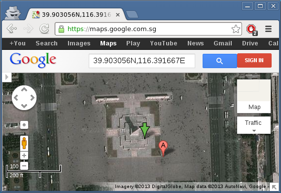
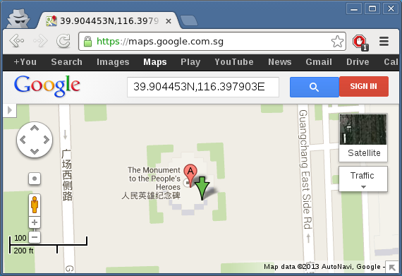
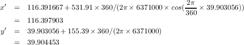
To check their correctness, we can compute a deviated coordinate and check whether it aligns with the deviated map. We now compute the deviated coordinate of the Monument to the People’s Heroes using its true coordinate (116.391667,39.903056).4 fx(116.391667,39.903056) = 531.91 meters and fy(116.391667,39.903056) = 155.39 meters. This means that the deviated coordinate is 531.91 meters to the east and 155.39 to the north. We then convert meters into degrees and adds them to the true coordinate.

x′  =  116.391667 + 531.91× 360∕(2π× 6371000× cos( 2π-× 39.903056))
                                                360
    =  116.397903
y′  =  39.903056 + 155.39× 360∕(2π× 6371000)
    =  39.904453


PIC


Figure 8: The monument’s true coordinate in GMap’s satellite image


PIC


Figure 9: The monument’s deviated coordinate in GMap’s street map


The green arrow in Figure 8 shows the true coordinate in the Google Maps’ satellite image. Figure 9 shows the deviated coordinate in the Google Maps’ street map. The red balloon, which is the nearest landmark, should be ignored. The green arrows in both maps are slightly to the southeast of the monument center, but as long as they offset the same amount, it is as good.